Weibull distribution
| Probability density function |
|
| Cumulative distribution function |
|
| Parameters |  scale (real) scale (real) shape (real) shape (real) |
|---|---|
| Support |  |
 |
|
| CDF | 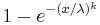 |
| Mean | 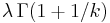 |
| Median |  |
| Mode | 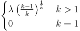 |
| Variance | 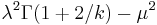 |
| Skewness | 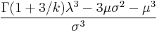 |
| Ex. kurtosis | (see text) |
| Entropy | 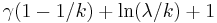 |
| MGF | 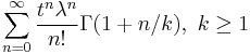 |
| CF | 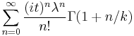 |
In probability theory and statistics, the Weibull distribution is a continuous probability distribution. It is named after Waloddi Weibull, who described it in detail in 1951, although it was first identified by Fréchet (1927) and first applied by Rosin & Rammler (1933) to describe the size distribution of particles.
Contents |
Definition
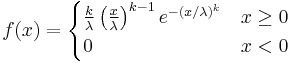
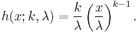
The probability density function of a Weibull random variable x is:[1]
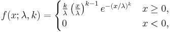
where k > 0 is the shape parameter and λ > 0 is the scale parameter of the distribution. Its complementary cumulative distribution function is a stretched exponential function. The Weibull distribution is related to a number of other probability distributions; in particular, it interpolates between the exponential distribution (k = 1) and the Rayleigh distribution (k = 2).
If the quantity x is a "time-to-failure", the Weibull distribution gives a distribution for which the failure rate is proportional to a power of time. The shape parameter, k, is that power plus one, and so this parameter can be interpreted directly as follows:
- A value of k<1 indicates that the failure rate decreases over time. This happens if there is significant "infant mortality", or defective items failing early and the failure rate decreasing over time as the defective items are weeded out of the population.
- A value of k=1 indicates that the failure rate is constant over time. This might suggest random external events are causing mortality, or failure.
- A value of k>1 indicates that the failure rate increases with time. This happens if there is an "aging" process, or parts that are more likely to fail as time goes on.
In the field of materials science, the shape parameter k of a distribution of strengths is known as the Weibull modulus.
Properties
Density function
The form of the density function of the Weibull distribution changes drastically with the value of k. For 0 < k < 1, the density function tends to ∞ as x approaches zero from above and is strictly decreasing. For k = 1, the density function tends to 1/λ as x approaches zero from above and is strictly decreasing. For k > 1, the density function tends to zero as x approaches zero from above, increases until its mode and decreases after it. It is interesting to note that the density function has infinite negative slope at x=0 if 0 < k < 1, infinite positive slope at x= 0 if 1 < k < 2 and null slope at x= 0 if k > 2. For k= 2 the density has a finite positive slope at x=0. As k goes to infinity, the Weibull distribution converges to a Dirac delta distribution centred at x= λ. Moreover, the skewness and coefficient of variation depend only on the shape parameter.
Distribution function
The cumulative distribution function for the Weibull distribution is
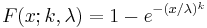
for x ≥ 0, and F(x; k; λ) = 0 for x < 0.
The failure rate h (or hazard rate) is given by
Moments
The moment generating function of the logarithm of a Weibull distributed random variable is given by[2]
![E\left[e^{t\log X}\right] = \lambda^t\Gamma\left(\frac{t}{k}%2B1\right)](/2012-wikipedia_en_all_nopic_01_2012/I/09f9eb866b30f9e927f35eebf4029827.png)
where Γ is the gamma function. Similarly, the characteristic function of log X is given by
![E\left[e^{it\log X}\right] = \lambda^{it}\Gamma\left(\frac{it}{k}%2B1\right).](/2012-wikipedia_en_all_nopic_01_2012/I/a62a6b02fb7e0b1a86dc3de44799454e.png)
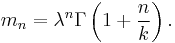
In particular, the nth raw moment of X is given by
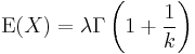
The mean and variance of a Weibull random variable can be expressed as
and
![\textrm{var}(X) = \lambda^2\left[\Gamma\left(1%2B\frac{2}{k}\right) - \Gamma^2\left(1%2B\frac{1}{k}\right)\right]\,.](/2012-wikipedia_en_all_nopic_01_2012/I/f7c95c93bf51d2722a76916f81377acb.png)
The skewness is given by
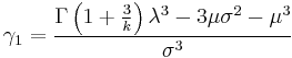
where the mean is denoted by μ and the standard deviation is denoted by σ.
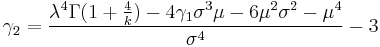
The excess kurtosis is given by
![\gamma_2=\frac{-6\Gamma_1^4%2B12\Gamma_1^2\Gamma_2-3\Gamma_2^2
-4\Gamma_1\Gamma_3%2B\Gamma_4}{[\Gamma_2-\Gamma_1^2]^2}](/2012-wikipedia_en_all_nopic_01_2012/I/642e218125f24368120e15265357cdc1.png)
where  . The kurtosis excess may also be written as:
Moment generating function
A variety of expressions are available for the moment generating function of X itself. As a power series, since the raw moments are already known, one has
![E\left[e^{tX}\right] = \sum_{n=0}^\infty \frac{t^n\lambda^n}{n!}\Gamma\left(1%2B\frac{n}{k}\right).](/2012-wikipedia_en_all_nopic_01_2012/I/91cc955f8bacc3a11e478ed925256ae3.png)
Alternatively, one can attempt to deal directly with the integral
![E\left[e^{tX}\right] = \int_0^\infty e^{tx} \frac{k}{\lambda}\left(\frac{x}{\lambda}\right)^{k-1}e^{-(x/\lambda)^k}\,dx.](/2012-wikipedia_en_all_nopic_01_2012/I/404beeb55e8dae10aca381fbf1324f74.png)
If the parameter k is assumed to be a rational number, expressed as k = p/q where p and q are integers, then this integral can be evaluated analytically.[3] With t replaced by −t, one finds
![E\left[e^{-tX}\right] = \frac1{ \lambda^k\, t^k} \, \frac{ p^k \, \sqrt{q/p}} {(\sqrt{2 \pi})^{q%2Bp-2}} \, G_{p,q}^{\,q,p} \!\left( \left. \begin{matrix} \frac{1-k}{p}, \frac{2-k}{p}, \dots, \frac{p-k}{p} \\ \frac{0}{q}, \frac{1}{q}, \dots, \frac{q-1}{q} \end{matrix} \; \right| \, \frac {p^p} {\left( q \, \lambda^k \, t^k \right)^q} \right)](/2012-wikipedia_en_all_nopic_01_2012/I/f802b86cb572a45d69a85cfab2222ea4.png)
where G is the Meijer G-function.
The characteristic function has also been obtained by Muraleedharan et al. (2007).
Information entropy
The information entropy is given by
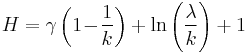
where  is the Euler–Mascheroni constant.
Weibull plot
The goodness of fit of data to a Weibull distribution can be visually assessed using a Weibull Plot.[4] The Weibull Plot is a plot of the empirical cumulative distribution function  of data on special axes in a type of Q-Q plot. The axes are
  versus
  . The reason for this change of variables is the cumulative distribution function can be linearised:
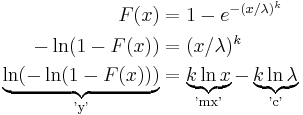
which can be seen to be in the standard form of a straight line. Therefore if the data came from a Weibull distribution then a straight line is expected on a Weibull plot.
There are various approaches to obtaining the empirical distribution function from data: one method is to obtain the vertical coordinate for each point using 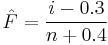 where
where  is the rank of the data point and
  is the number of data points.[5]
Linear regression can also be used to numerically assess goodness of fit and estimate the parameters of the Weibull distribution. The gradient informs one directly about the shape parameter  and the scale parameter
  can also be inferred.
Uses
The Weibull distribution is used
- In survival analysis[6]
- In reliability engineering and failure analysis
- In industrial engineering to represent manufacturing and delivery times
- In extreme value theory
- In weather forecasting
- To describe wind speed distributions, as the natural distribution often matches the Weibull shape[7]
- In communications systems engineering
- In radar systems to model the dispersion of the received signals level produced by some types of clutters
- To model fading channels in wireless communications, as the Weibull fading model seems to exhibit good fit to experimental fading channel measurements
- In General insurance to model the size of Reinsurance claims, and the cumulative development of Asbestosis losses
- In forecasting technological change (also known as the Sharif-Islam model)
- In hydrology the Weibull distribution is applied to extreme events such as annual maximum one-day rainfalls and river discharges. The blue picture illustrates an example of fitting the Weibull distribution to ranked annually maximum one-day rainfalls showing also the 90% confidence belt based on the binomial distribution. The rainfall data are represented by plotting positions as part of the cumulative frequency analysis.
- In describing the size of particles generated by grinding, milling and crushing operations, the 2-Parameter Weibull distribution is used, and in these applications it is sometimes known as the Rosin-Rammler distribution. In this context it predicts fewer fine particles than the Log-normal distribution and it is generally most accurate for narrow particle size distributions. The interpretation of the cumulative distribution function is that F(x; k; λ) is the mass fraction of particles with diameter smaller than x, where λ is the mean particle size and k is a measure of the spread of particle sizes.
Related distributions
- The translated Weibull distribution contains an additional parameter.[2] It has the probability density function
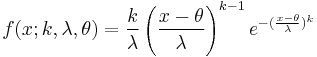
for  and f(x; k, λ, θ) = 0 for x < θ, where
  is the shape parameter,
  is the scale parameter and
  is the location parameter of the distribution. When θ=0, this reduces to the 2-parameter distribution.
- The Weibull distribution can be characterized as the distribution of a random variable X such that the random variable
is the standard exponential distribution with intensity 1.[2]
- The Weibull distribution interpolates between the exponential distribution with intensity 1/λ when k = 1 and a Rayleigh distribution of mode
 when k = 2.
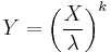
- The Weibull distribution can also be characterized in terms of a uniform distribution: if X is uniformly distributed on (0,1), then the random variable
 is Weibull distributed with parameters k and λ. This leads to an easily implemented numerical scheme for simulating a Weibull distribution.
- The Weibull distribution (usually sufficient in reliability engineering) is a special case of the three parameter Exponentiated Weibull distribution where the additional exponent equals 1. The Exponentiated Weibull distribution accommodates unimodal, bathtub shaped*[8] and monotone failure rates.
- The Weibull distribution is a special case of the generalized extreme value distribution. It was in this connection that the distribution was first identified by Maurice Fréchet in 1927. The closely related Fréchet distribution, named for this work, has the probability density function

- The Weibull distribution can also be generalized to the 3 parameter exponentiated Weibull distribution. This models the situation when the failure rate of a system is due to a combination of factors, and may increase for some times and decrease for other times (see bathtub curve).
- The distribution of a random variable that is defined as the minimum of several random variables, each having a different Weibull distribution, is a poly-Weibull distribution.
See also
References
- ^ Papoulis, Pillai, "Probability, Random Variables, and Stochastic Processes, 4th Edition
- ^ a b c Johnson, Kotz & Balakrishnan 1994
- ^ See (Cheng, Tellambura & Beaulieu 2004) for the case when k is an integer, and (Sagias & Karagiannidis 2005) for the rational case.
- ^ The Weibull plot
- ^ Wayne Nelson (2004) Applied Life Data Analysis. Wiley-Blackwell ISBN 0471644625
- ^ Survival/Failure Time Analysis
- ^ Wind Speed Distribution Weibull
- ^ "System evolution and reliability of systems". Sysev (Belgium). 2010-01-01. http://www.sys-ev.com/reliability01.htm.
Bibliography
- Fréchet, Maurice (1927), "Sur la loi de probabilité de l'écart maximum", Annales de la Société Polonaise de Mathematique, Cracovie 6: 93–116.
- Johnson, Norman L.; Kotz, Samuel; Balakrishnan, N. (1994), Continuous univariate distributions. Vol. 1, Wiley Series in Probability and Mathematical Statistics: Applied Probability and Statistics (2nd ed.), New York: John Wiley & Sons, ISBN 978-0-471-58495-7, MR1299979
- Muraleedharan, G.; Rao, A.G.; Kurup, P.G.; Nair, N. Unnikrishnan; Sinha, Mourani (2007), "Coastal Engineering", Coastal Engineering 54 (8): 630–638, doi:10.1016/j.coastaleng.2007.05.001
- Rosin, P.; Rammler, E. (1933), "The Laws Governing the Fineness of Powdered Coal", Journal of the Institute of Fuel 7: 29–36.
- Sagias, Nikos C.; Karagiannidis, George K. (2005), "Gaussian class multivariate Weibull distributions: theory and applications in fading channels", Institute of Electrical and Electronics Engineers. Transactions on Information Theory 51 (10): 3608–3619, doi:10.1109/TIT.2005.855598, ISSN 0018-9448, MR2237527
- Weibull, W. (1951), "A statistical distribution function of wide applicability", J. Appl. Mech.-Trans. ASME 18 (3): 293–297, http://www.barringer1.com/wa_files/Weibull-ASME-Paper-1951.pdf.
- "Engineering statistics handbook". National Institute of Standards and Technology. 2008. http://www.itl.nist.gov/div898/handbook/eda/section3/eda3668.htm.
- Nelson, Jr, Ralph (2008-02-05). "Dispersing Powders in Liquids, Part 1, Chap 6: Particle Volume Distribution". http://www.erpt.org/014Q/nelsa-06.htm. Retrieved 2008-02-05.
External links
|
|||||||||||